Optimal sensors placement in the Arctic
For a high-precision operational ocean state forecast, there is a need for regular expensive measurements, so an optimal configuration of the observing system is needed. In the course of our research, we are developing a method for finding the optimal coordinates of meters using machine learning methods, which consists of two stages: at the first stage, an approximation of the information entropy field is performed, at the second stage, the information entropy field is used to initialize the binary mask of the continual autoencoder, and the corresponding sensor locations are further optimized, to maximize the accuracy of physical field reconstruction and minimize the total number of sensors. The proposed method is described in more detail in the article (Turko et al, 2022). Here, the results are presented of a study on the effectiveness of the proposed method in comparison with some well-known methods (principal component analysis with QR factorization - PCA-QR) and benchmarks (mean climatic value).
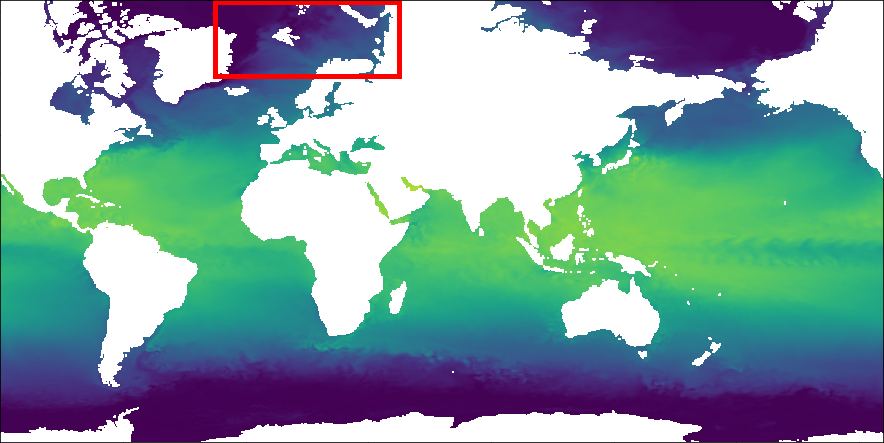
Figure 1. Selected region near Svalbard archipelago chosen for consideration
A small region around the Svalbard archipelago was chosen for the study (figure 1) with a computational grid size of 300x120 cells in the horizontal plane. The size of the region was selected due to the scaling limitations of the PCA-QR method, which includes SVD decomposition, the execution time of which grows cubically with the number of cells.
Figure 2 shows the information entropy fields calculated from the testset with the selected smoothing for the temperature and salinity fields in the near-surface and deep layers. The color indicates the value of information entropy in nats per cell of the computational grid. The value characterizes the average level of "uncertainty" inherent in the possible outcomes of the variable. A small value means that we had more a priori information about the temperature at this point than at a point with a higher information entropy. The result obtained is consistent with the hydrophysics of the region under consideration.
Examples of the reconstructed fields are shown in figure 3. Accuracy calculated using the Bias and RMSE formulas are shown in figure 4, with median values. The corresponding time series is shown in figure 5. And the final values of the recovery accuracy are presented in table 1. The proposed coordinates of the samplers are marked with red dots in figures 3, 4.
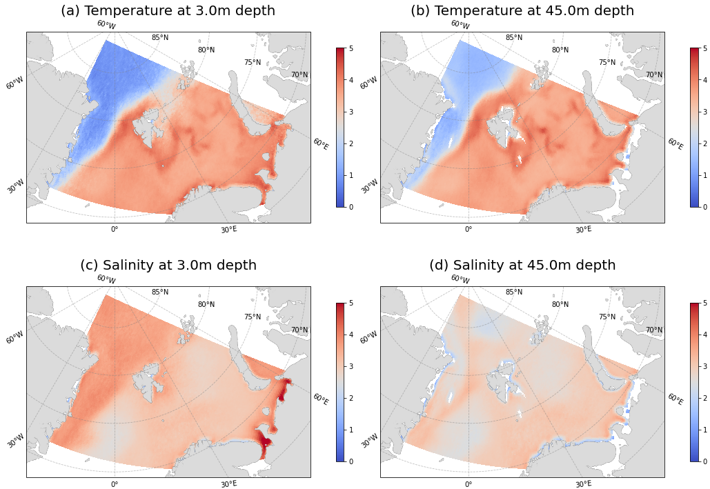
Figure 2. Smoothed ensemble mean information entropy of geophysical fields: temperature at (a) 3 meter and (b) 45 m depth; salinity at (c) 3 meter and (d) 45 m depth
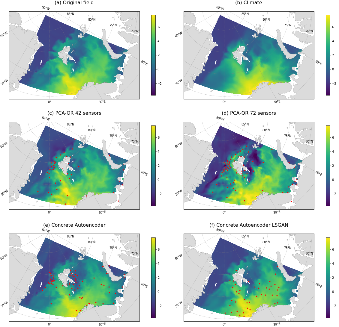
Figure 3. Reconstructed temperature fields at 45 m depth, 7 Aug 2017
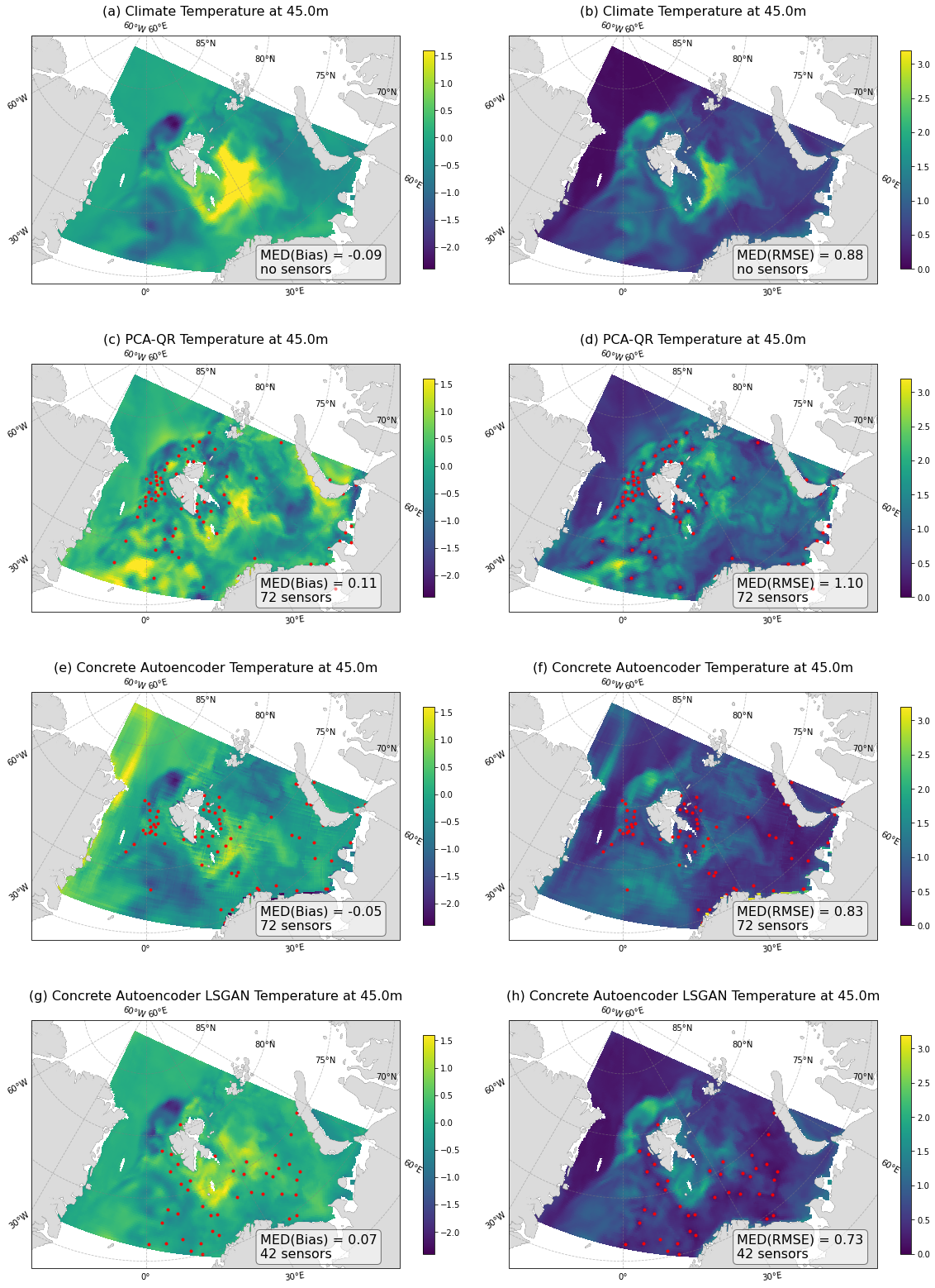
Figure 4. Temperature field reconstruction based on measurements accuracy against original model data. Bias/RMSE temperature reconstruction at depth 45m by methods: (a)/(b) Climate, (c)/(d) PCA-QR, (e)/(f) Concrete Autoencoder, (g)/(h) Concrete Autoencoder with LSGAN. At the left corner of each plot shown the time median field value and the number of measurements
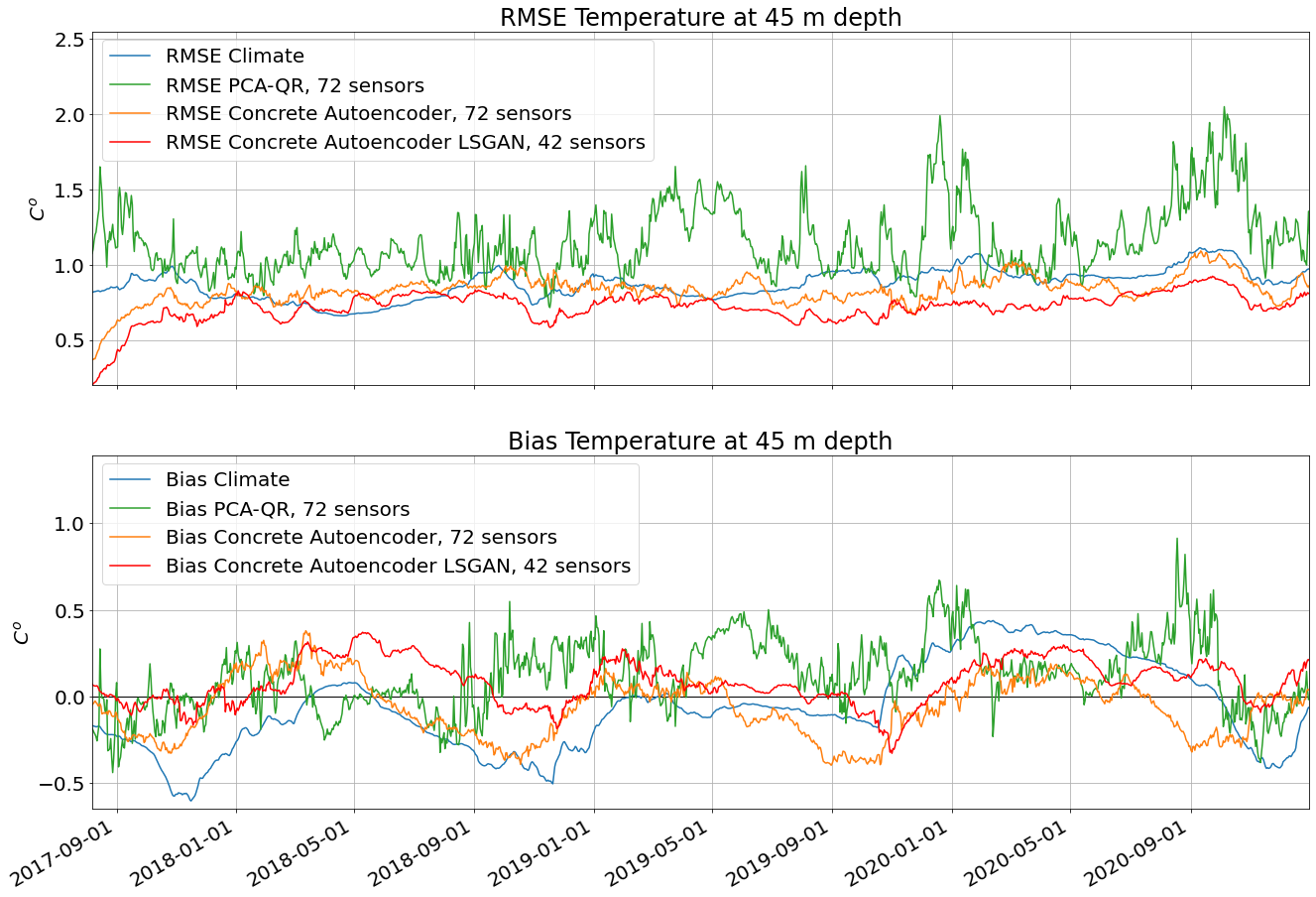
Figure 5. Temperature field reconstruction accuracy against original model data. RMSE/Bias time series based on data from the test dataset
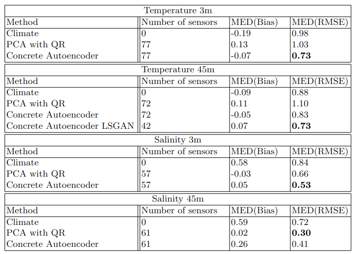
Table 1. Test set reconstruction errors
Literature
Turko, N., Lobashev, A., Ushakov, K., Kaurkin, M., Ibrayev, R. (2022). Information Entropy Initialized Concrete Autoencoder for Optimal Sensor Placement and Reconstruction of Geophysical Fields. In: Voevodin, V., Sobolev, S., Yakobovskiy, M., Shagaliev, R. (eds) Supercomputing. RuSCDays 2022 Lecture Notes in Computer Science, vol 13708 Springer, Cham. https://doi.org/10.1007/978-3-031-22941-1_12
